Metabarcoding data analysis quick start guide

Ohio Supercomputer Center (OSC) Batch System Basics
1.1 How It Works
1.2 Advantages of Batch Systems Over Interactive Sessions
Pre-DADA2 Steps
DADA2
Phyloseq

Ohio Supercomputer Center (OSC) Batch System Basics

The OSC uses Slurm, a batch system scheduler, to manage tasks on shared supercomputer clusters.

How It Works:

1. Write a job script

Define your task (e.g., simulations, data analysis).
Specify required resources (CPUs, memory, runtime) using #SBATCH directives.

Example script (myjob.sh):

#!/bin/bash
#SBATCH --time=2:00:00  
#SBATCH --nodes=1  
my_program  

2. Submit the job

Run sbatch myjob.sh in the terminal to add it to the queue.
3. Retrieve results
Outputs are saved to files (e.g., myjob.log).
Advantages of Batch Systems Over Interactive Sessions
Efficiency: Automatically runs jobs during idle periods (e.g., nights/weekends).
Scalability: Manages long/large jobs without active monitoring.
Reproducibility: Scripts ensure identical setups for reruns.
Priority: Slurm optimizes cluster throughput by prioritizing short/urgent jobs.

In short, we run the scripts through a terminal rather than R Studio. Batch processing also allows us to run different programs in single bash script. for eg: FIGARO is python based and DADA2 is R based, we can run both programs in the same batch script as single job.

Pre-DADA2 Steps

1. Organizing Input Data.

Prerequisites:

Raw FASTQ files: Ensure files are named in the standard fastq format.
Primer Info: Specific information for the gene (e.g., 16S) and region (e.g., V4). sequence and length.
Reference Databases: Download SILVA (16S) and PR2 (18S).# Check for updates regularly.

Illumina naming format : The Illumina instruments follow a unified file naming system to demultiplexed reads which helps to identify reads origin.

Example file name:
WLE-T3S3-0-1A-16S-V4_S71_L001_R1_001.fastq.gz

Component	Description
`WLE-T3S3-0-1A`	Sample ID
`16S`	Target gene (16S rRNA)
`V4`	Variable region
`S71`	Sample number in loading sheet
`L001`	Flow cell lane
`R1`/`R2`	Forward/Reverse read
`001`	its always 001 and I don’t know why

If you have reads for each of your samples means the data is demultiplexed.

2. Separating reads based on Samples/Gene/Variable regions.

The sequencing facility can run multiple samples with multiple regions (16S and 18S) in the same run, so the first step in the analysis will be separating data based on the need. Separate the files using grouping16S_18S.R script.

Tip: if you follow the pattern ( /users/PJSXXXX/USER_NAME/Data/SAMPLE_PROJECT_NAME/GENE_NAME/VAR_REGION), it will be easier to rename paths without error.
Source: “/users/PJS/USER_NAME/Data/WLO/16S/V4/”
Figures: “/users/PJS/USER_NAME/Data/WLO/16S/V4/Figures”

If you follow the same format, file paths can be defined by changing the USER_NAME with your username. Press Ctrl+H to open find and replace dialogue box.

source_dir <- define the folder address where you have all you raw reads (the folder downloaded from sequencing facility website).

The first part of the script is a function to move files with specified word or letters(pattern) in the filename to a specified folder.

move_files("18S", "18S") : the first “18S” denotes the word (pattern) that we need to separate (for all 18S reads, the file name contain 18S. The second “18S” denotes the destination folder name.

Other scenarios: If the sequences are of 18S reads from two different sites eg: WLO and WLE, the pattern will be the names of samples.
If the sequences are from two regions of 18S (V7 and V9) from different samples, rerun the codes until desired level of separation is obtained.

eg: If the source folder contains following files:
WLE-T3S3-0-1A-16S-V4_S71_L001_R1_001.fastq.gz
WLE-T3S3-0-1A-16S-V4_S71_L001_R2_001.fastq.gz
WLE-T3S3-0-1A-16S-V9_S71_L001_R1_001.fastq.gz
WLE-T3S3-0-1A-16S-V9_S71_L001_R2_001.fastq.gz
WLO-T3S3-0-1A-16S-V4_S71_L001_R1_001.fastq.gz
WLO-T3S3-0-1A-16S-V4_S71_L001_R2_001.fastq.gz
WLO-T3S3-0-1A-16S-V9_S71_L001_R1_001.fastq.gz
WLO-T3S3-0-1A-16S-V9_S71_L001_R2_001.fastq.gz
WLE-T3S3-0-1A-18S-V4_S71_L001_R1_001.fastq.gz
WLE-T3S3-0-1A-18S-V4_S71_L001_R2_001.fastq.gz
WLE-T3S3-0-1A-18S-V9_S71_L001_R1_001.fastq.gz
WLE-T3S3-0-1A-18S-V9_S71_L001_R2_001.fastq.gz
WLO-T3S3-0-1A-18S-V4_S71_L001_R1_001.fastq.gz
WLO-T3S3-0-1A-18S-V4_S71_L001_R2_001.fastq.gz
WLO-T3S3-0-1A-18S-V9_S71_L001_R1_001.fastq.gz
WLO-T3S3-0-1A-18S-V9_S71_L001_R2_001.fastq.gz

Workflow will be:

Step 1: Separate samples by location:

move_files("WLE", "WLE")  # Moves WLE samples to a "WLE" folder
move_files("WLO", "WLO")  # Moves WLO samples to a "WLO" folder

Step 2: Split 16S and 18S reads:

move_files("16S", "16S")  # Moves 16S reads to a "16S" folder  
move_files("18S", "18S")  # Moves 18S reads to an "18S" folder

Step 3: Separate variable regions (V4/V9):

move_files("V4", "V4")  # Moves V4 reads to a "V4" folder  
move_files("V9", "V9")  # Moves V9 reads to a "V9" folder

make sure all the files are grouped accordingly.

DO NOT process different regions (V4/V9) together.

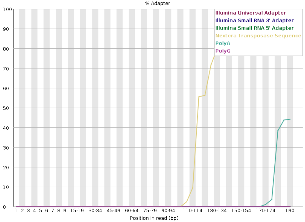
The demuxed reads still might contain sequencing artifacts like adapters and primers. To check the quality of raw fastq files, FastQC is used.

2. FastQC - QC check

To run FastQC on OSC:

module load fastqc/0.12.1
mkdir ~/16S/fastQC_out
cd ~/16S/
fastqc -o ~/16S/fastQC_out *.fastq.gz

The script runs import FastQC module on OSC cluster # Note the versions might changes use module spider fastqc to find latest loading script.
The mkdir cmd creates output directory for fastqc results which are in .html format. Make sure you are providing correct file paths to fastqQC_out folder and you are in the folder containing raw reads while running fastqc.

More info

FastQC example output for reads with adapter contamination.

FastQC

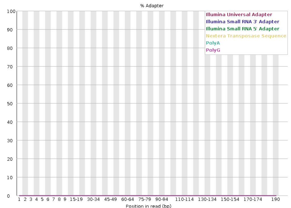
FastQC example output for reads without adapter contamination.

FastQC

FastQC generates outputs in .html and .zip formats. .zip files can be removed using remove_files.sh to save space.

5. Removing adapter bases using `Cutadapt`.

From FastQC results, the adapter presence can be determined.

Installation of Cutadapt

Run the following scripts on Terminal (It’s better to run this on an interactive session)

module load miniconda3/24.1.2-py310
conda config --add channels bioconda
conda config --add channels conda-forge
conda create -n cutadapt cutadapt
conda activate cutadapt
cutadapt --version

Once installed, you no longer need to run the above lines every time.

Running Cutadapt

cutadapt code:

-a "$ADAPTER_SEQ" -A "$ADAPTER_SEQ" \
-o "$trimmed_forward" -p "$trimmed_reverse" \
"$forward_read" "$reverse_read" \
--length 200 --length 200 \
--minimum-length 200  

-a : adapter
-A : adapter
-o : forward output
-p : reverse output
--length : trimming length
--minimum-length: discard reads below this length.

To run on OSC clusters, adjust the following parameters on cutadapt_16S.sh file.

INPUT_DIR="Data/OSG/16S"
OUTPUT_DIR="Data/OSG/16S/Cutadapt_out"
ADAPTER_SEQ="CTGTCTCTTATA" # If using kits other than Nextera, change sequence accordingly.

After this step, use FastQC.sh on output files to confirm adapter sequences are removed.

Determining truncation length (Can be omitted, if Sequences are trimmed during `Cutadapt` step)

In the DADA2 pipeline, truncation length determines where sequencing reads are trimmed to exclude regions where Q30 scores—indicating a base call accuracy of 99.9%—are no longer maintained, a crucial consideration for Illumina data. Since Q30 values often decline toward read ends in Illumina sequencing, truncation ensures error-prone regions (below Q30) are removed before denoising. This step refines DADA2’s error model by retaining only high-confidence bases, reducing the risk of inferring erroneous amplicon sequence variants (ASVs). Proper truncation also preserves high-quality overlap regions (Q30 or above) in paired-end reads, enabling accurate merging and reconstruction of full-length amplicons. Striking the right balance is essential: truncating too early may discard valid Q30 data, while truncating too late retains sub-Q30 bases that introduce noise. Optimizing truncation length thus maximizes both data integrity and taxonomic resolution, ensuring downstream analyses reflect true biological diversity. To ensure reproducibility and accuracy, a software called FIGARO is used in this pipeline. FIGARO determines the appropriate truncation length by analyzing the reads. If you are using FIGARO for first time run Figaro_Install.sh on OSC Cluster terminal using the command sbatch Figaro_Install.sh (change the code according to the file location eg: if the Figaro_Install.sh is in a folder named Codes, the code will be sbatch Codes/Figaro_Install.sh)

More info

NOTE: Before running FIGARO, adjust -f, -r, and -a values accordingly.

FIGARO analyze the raw reads and stores suggested truncation parameters as a .json file. The file contains the most suitable values as the first entry, so to pass these values to DADA2 in R, the .json file is imported to R and values are extracted.

DADA2

Currently we have raw reads grouped based on sample/gene/variable region. Our aim is to cluster reads based on similarity (100% for ASVs), then choose a representative sequence (ASVs) for each of these clusters and assign taxonomy using a reference database, then create a table showing the total number of each ASV in each sample and it’s taxonomy.

The script file DADA2_16S.R/DADA2_18S.R contains the complete DADA2 analysis pipeline. Before submitting the job at OSC, make necessary changes in the script file.

1. Change all the paths according to your environments

Make sure the file paths are defined correctly. The DADA2 starts working from the folder containing raw .fastq.gz files.

path <-"/users/PJS***/shantom/Data/WLO/16S" adjust the path according to your folder address.

Defining sample names: Sample names are extracted from fastq file names and assigned to the object sample.names by following line of code.

sample.names <- sapply(strsplit(basename(fnFs), "-16S"), [, 1)

if the fastq file name is WLE-T3S3-0-1A-16S-V4_S71_L001_R1_001.fastq.gz, the sample name will be the characters before the string “-16S”, which is WLE-T3S3-0-1A. The character string need to be changed according to the file names.

2. Error plotting

plotQualityProfile function in DADA2 plots the quality of reads in each sample (these images can used for QC, reads with values below Q30 might need rerun).

3. Filtering and Trimming

filterAndTrim function removes low quality reads and base pairs.

fnFs, filtFs, fnRs, filtRs: These are the inputs and outputs.
trimLeft=c(19,20): This values indicate the primer length and removes the indicated number of base pairs from reads, change according to primers.
truncLen=c(200,190): The truncation lengths after cutadapat,

4. Merging

The forward and reverse reads are merged together and this is used for further analysis. seqtab <- seqtaball[,nchar(colnames(seqtaball)) %in% 245:255]: This particular step allows to remove merged reads with lengths longer than expected.

5. Chimera removal

Merging might cause the formation of non-biological reads which are removed by removeBimeraDenovo.

6. QC check

The read retention rate can be analyzed at this step. Samples that have a rate below ~48% might need re-sequencing. The object track contains the number of reads passed after each of the above steps.

7. Taxonomy assignment

The taxonomy of representative sequences (ASVs) are assigned using a reference database.

For 16S, SILVA database is used.
For 18S, PR2 is used.

PR2 and SILVA has different taxonomical ranks, so the code needs to be adjusted.

16S: taxa <- assignTaxonomy(seqtab.nochim, "~/silva_nr99_v138.1_wSpecies_train_set.fa.gz", multithread=TRUE)  

18S: taxa <- assignTaxonomy(seqtab.nochim, "~/pr2_version_5.0.0_SSU_dada2.fasta.gz", multithread=TRUE, 
        taxLevels=c("Domain", "Supergroup", "Division","Subdivision", "Class", "Order", "Family", "Genus", "Species"))

8. Excel files

A set of tables are created using the excel conversion scripts. The file with .xlsx ext contain all the tables and can be used to have an overall understanding of the data. (NOTE: This file contains all the data and not decontaminated so DO NOT USE this file for analysis).

9. Phyloseq

DADA2 pipeline identifies species taxonomy from the raw sequence reads and number of reads belongs to each species (ASV). To analyze microbial community following components are needed:
1. ASV table (count table)
2. Taxonomy table
3. Representative sequences
4. Phylogenetic tree
5. Metadata

To analyze/interpret microbial community structure , all these different objects need to be processed as a single object in R.
PHYLOSEQ combines all these different data objects to a single object to make the computation process easier.
DADA2 produced ASV table, Taxonomy table and Representative sequences. We need to construct phylogenetic tree from the representative sequences and provide a metadata file to proceed with PHYLOSEQ analysis.
PHYLOSEQ analysis use less computing power and can be run from laptops (after decontamination and phylogenetic tree construction).

10. Metadata file

The script produces a template for metadata file, which can be edited to add all available info for the samples. Apart from the collected information, 2 additional columns (denoting controls) need to be added for use with decontam package.

SampleID	Sample_or_Control	Keep	MetaData1	MetaData2
Blank	Control	No	NA	NA
WLE-T3S3	Sample	Yes	2.1	June
WLE-T3S3	Sample	Yes	2.1	May

IMPORTANT NOTE: The metadata file included in the folder is only a template. Make sure to replace it with your own edited metadata file.

Note: While writing the code for OSG, I included some non-blank samples that needed to be removed later. To handle this, I added a Keep column to indicate which samples should be retained. You can remove this column if only blank samples need to be excluded. However, if any samples fail the rarefaction QC, simply set their Keep value to No to exclude them.

Phyloseq

The second step of workflow is running Phyloseq.sh script in terminal to execute Phyloseq.R script.

1. Decontamination

The possible contamination occurred during wet lab workflow is removed by comparing reads produced from blank samples (In theory, these samples shouldn’t produce any reads). Decontam package compares the prevalence of possible contaminant reads from blanks to samples and remove such reads.

NOTE : Make sure correct metadata file is supplied (any error in metadata file will result in job failure or improper result interpretation).

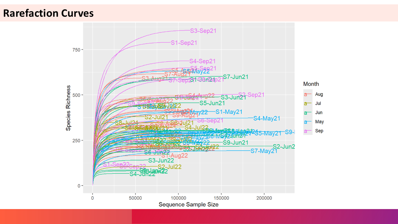
2. Rarefaction QC

Rarefaction curves are used to check whether the sequencing depth (number of reads) was sufficient to recover most of the species. The flattening of the curves indicate that most of the species present in the community is recovered and increasing sequencing depth will not yield new species. The steep curves that doesn’t get flattened out indicate the opposite of the above and such samples should removed from further analysis.

Rarefaction Curves

3. Tidying the `Phyloseq` Object

After removing potential contaminants and obtaining rarefaction curves, blank samples and those that failed rarefaction QC can be excluded from the Phyloseq object. At this stage, I also remove eukaryotic, mitochondrial, and chloroplast reads from the 16S dataset, as well as bacterial reads from the 18S dataset. Additionally, removing samples may leave ASVs in the ASV table that were present only in those samples. These ASVs can also be filtered out at this stage.

4. Tree construction

Phylogenetic tree is needed for different analyses like UNIFRAC, Null Models etc. Tree building is computationally intensive (for 90 samples with 48 cores, it takes 8-12 hours), so request OSC resources according to your sample size.

fitGTR <- update(fit, k=4, inv=0.2) . I didn’t understand this step well. This code analyzes and refits the tree structure, with a small set I found that best-fit (from AIC(fitGTR) for a 2 sample WLO18S dataset is when k=4 and inv=0.5. But for higher sample counts, this step takes very long run times and often crashes in between. So start with fitGTR <- update(fit, k=4, inv=0.2), if it fails reduce k=2 and inv=0 then increase k and inv gradually until you reach the crashing point.

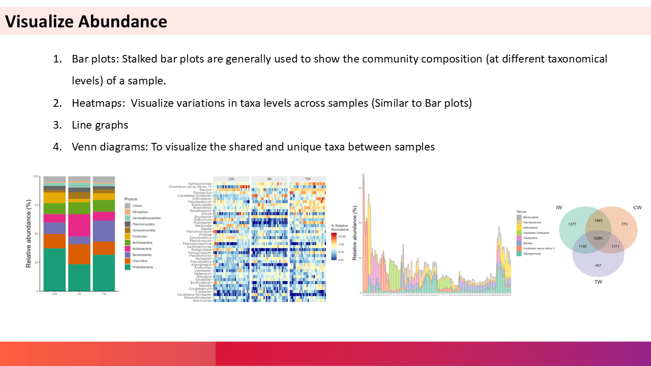
5. Community distribution across samples

To visualize community distribution across samples can be visualized using bar and line plots. They are useful in getting an overall idea and to see trends over samples (in time or space scales).

Community Distribution

6. Alpha Diversity

Alpha diversity measures the species diversity within a single sample or habitat. It reflects the richness (number of species), evenness (distribution of abundances), and/or phylogenetic diversity of organisms in a community.

6.1 Chao1

A non-parametric estimator of species richness, Chao1 predicts the total number of species in a community, including undetected rare species. It is particularly useful for datasets with many rare taxa (e.g., microbiome studies). This metric uses singletons and doubletons in the dataset. DADA2 often removes singletons and doubletons during the analysis, so Chao1 is NOT RECOMMENDED for DADA2 derived datasets.

6.2 Shannon Index

The Shannon Index (or Shannon-Wiener/Shannon-Weaver index) quantifies diversity by accounting for both species richness and evenness. Higher values indicate greater diversity, calculated as:
H' = -Σ(p_i * ln(p_i)), where p_i is the proportion of species i.

6.3 Simpson Index

The Simpson Index measures the probability that two randomly selected individuals belong to the same species. Values range from 0 (infinite diversity) to 1 (no diversity). Often reported as 1 - D or 1/D for intuitive interpretation.

#### 6.4 Faith’s PD Faith’s Phylogenetic Diversity (PD) incorporates evolutionary relationships by summing the total branch length of a phylogenetic tree spanning all species in a sample. It reflects both taxonomic and evolutionary diversity.

7. Beta Diversity

Beta diversity quantifies the differences in species composition between samples or habitats. It reflects how communities change across environmental gradients, geographic distances, or experimental conditions.

7.1 Bray-Curtis

Bray-Curtis dissimilarity measures compositional differences between samples based on species abundance data. It ranges from 0 (identical communities) to 1 (no shared species). Formula:
BC = 1 - (2 * Σ min(Abundance_i, Abundance_j) / (Σ Abundance_i + Σ Abundance_j))

7.2 Jaccard’s Index

Jaccard’s Index assesses similarity based on species presence/absence, ignoring abundance. Values range from 0 (no overlap) to 1 (identical species). Often used for binary (yes/no) community comparisons.

7.3 UniFrac

UniFrac incorporates phylogenetic relationships to measure community dissimilarity. It calculates the fraction of unique branch lengths in a phylogenetic tree between samples.

7.3.1 Weighted UniFrac

Accounts for species abundance and phylogenetic branch lengths. Sensitive to dominant taxa, making it ideal for detecting shifts in abundant lineages.

7.3.2 Unweighted UniFrac

Focuses solely on presence/absence and phylogenetic tree structure. Highlights differences in rare taxa or evolutionary distinctiveness.

8. Ordination Techniques

Ordination methods reduce complex ecological or multivariate data into a simplified visual space to reveal patterns. They are generally categorized as unconstrained (without external variables) or constrained (guided by external variables such as environmental data).

8.1 Unconstrained Methods

These techniques explore inherent patterns in the data without using explanatory variables.

8.1.1 PCA (Principal Component Analysis)

PCA is an unconstrained method that reduces dimensionality by transforming correlated variables into a set of linearly uncorrelated principal components. It is widely used for exploratory data analysis.

8.1.2 PCoA (Principal Coordinate Analysis)

PCoA, also known as metric multidimensional scaling, is an unconstrained method that visualizes dissimilarities between samples using distance metrics (e.g., Bray-Curtis, UniFrac).

8.1.3 NMDS (Non-Metric Multidimensional Scaling)

NMDS is an unconstrained method that ranks samples based on dissimilarity, preserving their relative distances in a low-dimensional space. It is robust for non-linear relationships.

8.2 Constrained Methods

These methods incorporate external explanatory variables (e.g., environmental factors) to directly model variation in the response data.

8.2.1 RDA (Redundancy Analysis)

RDA is a constrained ordination method that combines multiple regression with PCA. It models how much variation in the community data can be explained by specified predictors.

8.2.2 dbRDA (Distance-Based Redundancy Analysis)

dbRDA is a constrained extension of RDA that allows the use of any dissimilarity measure. It is often used with ecological data (e.g., Bray-Curtis, UniFrac) and requires explanatory variables.

9. Indicator Species Analysis

Indicator Species Analysis is a statistical method used to identify species that are significantly associated with specific groups of sites or environmental conditions. These species, known as indicator species, provide insights into ecological communities, habitat conditions, or environmental changes. The analysis is widely used in ecology, conservation biology, and environmental monitoring.

Indicator Value (IndVal): A metric that quantifies the strength of the association between a species and a group of sites. It combines specificity (how unique a species is to a group) and fidelity (how frequently it occurs in that group).

Statistical Significance: Permutation tests are often used to assess whether the observed indicator values are significant.

Applications:

Identifying species indicative of specific habitats or environmental gradients.
Monitoring ecosystem health and biodiversity.
Assessing the impact of environmental changes or management practices.

The indicspecies package in R provides tools for conducting indicator species analysis. It includes functions to calculate indicator values, perform permutation tests, and visualize results.

multipatt(): Identifies indicator species for combinations of site groups.

10. Dirichlet-Based Methods

Dirichlet-based approaches model compositional data using the Dirichlet distribution, a probability distribution over simplices (i.e., data where components sum to 1). These methods are widely used in microbiome studies to infer latent structures, such as microbial subcommunities or functional groups.

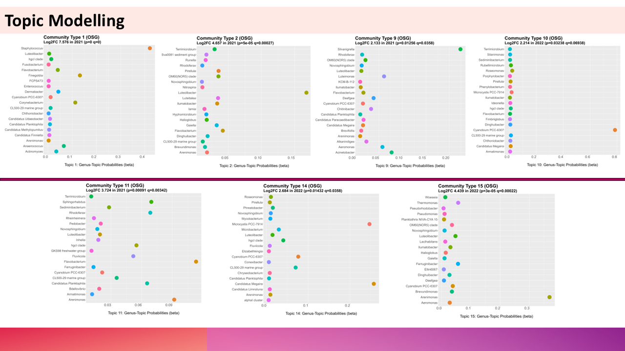
10.1 Topic Modelling

Topic modelling identifies latent “topics” (e.g., microbial subcommunities) in datasets by assuming each sample is a mixture of these topics. Analogous to text analysis:

Samples ≈ “Documents”
Microbial taxa ≈ “Words”
Topics ≈ Groups of co-occurring taxa (e.g., aerobic bacteria, sulfate-reducers).

Application in Microbiome Studies:

Detects recurring microbial assemblages across samples.
Reduces high-dimensional taxonomic data into interpretable subcommunities.

TopicModelling

10.2 Latent Dirichlet Allocation (LDA)

LDA is a specific Dirichlet-based topic model that assumes:

Each sample is a mixture of K latent topics.
Each topic is a Dirichlet-distributed mixture of taxa.

Key Components:

Dirichlet Prior (α): Controls topic sparsity across samples.
Dirichlet Prior (η): Controls taxon sparsity within topics.

Application in Microbial Analysis:

Identifies taxa that co-vary across samples (e.g., symbionts or competitors).
Quantifies how environmental factors (e.g., pH, diet) influence topic distributions.

Example:
Modeling soil microbiomes to uncover latent topics linked to nutrient gradients (e.g., nitrogen-rich vs. carbon-rich microbial consortia).

Why Use Dirichlet Models in Microbiome Studies?

Compositional Data: Naturally handles relative abundances (e.g., 16S rRNA amplicon data).
Uncertainty Quantification: Provides probabilistic membership of taxa to topics.
Interpretability: Topics map to ecologically meaningful subcommunities.

11. Null Model Analysis

Generates random communities by shuffling taxa occurrences within phylogenetic bins.
Compares observed vs. null expectation to infer dominant assembly mechanisms.

11.1 iCAMP (Infer Community Assembly Mechanisms by Phylogenetic bin-based null model analysis)**

iCAMP quantifies the relative contributions of ecological processes (e.g., selection, dispersal, drift) to microbial community assembly using phylogenetic binning and null models.

Key Features:

Phylogenetic Binning:
- Groups taxa into bins based on evolutionary relationships (e.g., using phylogenetic trees).
- Reduces bias from uneven phylogenetic sampling and improves null model accuracy.
Process Partitioning:
- Decomposes beta diversity into contributions from:
  - Homogeneous Selection (similar environmental pressures).
  - Heterogeneous Selection (divergent environmental pressures).
  - Dispersal Limitation (limited microbial movement).
  - Drift (stochastic population changes).
  - Homogenizing Dispersal (high dispersal rates).

Infer Community Assembly Mechanisms by Phylogenetic bin-based null model analysis

Generates random communities by shuffling taxa occurrences within phylogenetic bins.
Compares observed vs. null expectation to infer dominant assembly mechanisms.

Application in Microbial Ecology:

Identifies why communities differ across environments (e.g., soil vs. ocean microbiomes).
Reveals how processes like pH selection or geographic isolation shape community structure.

Example:
In a study of grassland microbiomes, iCAMP might show that homogeneous selection dominates in pH-stable soils, while dispersal limitation drives differences between isolated sites.

Phylogenetic resolution: Accounts for evolutionary relationships, critical for trait-based assembly.
Quantitative partitioning: Assigns exact percentages to each ecological process.
Scalability: Handles large microbiome datasets (e.g., 16S rRNA amplicon data).

12. Co-occurrence Networks

Co-occurrence networks infer potential ecological interactions (e.g., mutualism, competition) between microbial taxa based on their abundance patterns across samples. These networks help identify keystone taxa, functional modules, and community stability drivers.

12.1 Correlation-Based Networks

Constructed using pairwise correlation metrics (e.g., Pearson, Spearman) to identify taxa that co-vary.

Key Features:
- Simple to implement but prone to spurious edges due to compositional data biases.
- Often filtered by significance (e.g., p-value adjustment) and thresholding (e.g., r > 0.6).
Applications:
- Exploratory analysis of gut microbiota to identify taxa clusters linked to health/disease.
Limitations:
- Fails to distinguish direct vs. indirect interactions.
  Alternatives: Use SparCC (Sparsity-Corrected Correlation) for compositional data.

12.2 SPIEC-EASI (SParse InversE Covariance Estimation for Ecological Association and Statistical Inference)

A robust method designed for compositional microbiome data. Estimates conditional dependencies (direct interactions) using:

MB (Meinshausen-Bühlmann): Neighborhood selection for sparse networks.
glasso (Graphical Lasso): L1-penalized covariance matrix inversion.
Key Features:
- Accounts for compositionality via log-ratio transformations (e.g., CLR).
- Reduces false positives compared to correlation-based methods.
Applications:
- Identify gut microbiome interactions that are resistant to diet-induced changes.

12.3 FlashWeave

A machine learning-based method that detects direct and indirect associations in sparse microbial datasets.

Key Features:
- Handles compositionality and heterogeneous data (e.g., taxa + environmental variables).
- Uses statistical independence tests and adaptive thresholding.
- Computationally intensive but highly accurate for large datasets.
Applications:
- Uncovering soil microbiome interaction networks influenced by pH and nutrient gradients.
Strengths:
- Robust to noise and outperforms SPIEC-EASI in benchmark studies.

Method Comparison

Method	Pros	Cons
Correlation-Based	Fast, intuitive	Spurious edges, ignores compositionality
SPIEC-EASI	Robust to compositionality, fewer false positives	Requires tuning (e.g., lambda parameter)
FlashWeave	High accuracy, detects indirect links	Computationally slow for large datasets

Example Use Case
In a marine microbiome study:

FlashWeave identifies a keystone cyanobacterium linked to nitrogen cycling.
SPIEC-EASI reveals a competitive relationship between Prochlorococcus and Synechococcus.

13. Functional Diversity Prediction

Functional diversity prediction infers metabolic or ecological roles of microbial communities using taxonomic or genomic data. These tools bypass costly metagenomic sequencing but rely on reference databases and assumptions.

13.1 FAPROTAX

FAPROTAX maps 16S rRNA gene sequences to metabolic traits (e.g., nitrification, sulfate reduction) using a manually curated database of cultured prokaryotes.

Key Features:

Focuses on biogeochemical cycles (C, N, S) and habitat-specific functions.
Simple to use: Requires an OTU table (taxonomic abundances) as input.

Applications:

Predicting functional shifts in marine microbiomes under oxygen depletion.
Linking soil taxa to carbon degradation pathways.

Limitations:

Database bias: Limited to ~4600 prokaryotic taxa and well-studied functions.
Culturing bias: Excludes uncultured taxa and novel functions.
No strain-level resolution: Ignores functional variability within genera.

13.2 PICRUSt2 (Phylogenetic Investigation of Communities by Reconstruction of Unobserved States)

PICRUSt2 predicts functional potential (e.g., KEGG pathways, EC numbers) from 16S data by inferring gene families via phylogenetic placement.

Key Features:

Uses reference genome databases (e.g., GTDB, IMG) and hidden-state prediction.
Outputs pathway abundances linked to MetaCyc/KEGG annotations.

Applications:

Predicting gut microbiome contributions to host vitamin synthesis.
Comparing functional redundancy in soil vs. aquatic microbiomes.

Limitations:

Reference dependency: Accuracy depends on genome completeness and phylogenetic proximity to reference taxa.
Pipeline complexity: Requires precise OTU clustering (e.g., closed-reference) and alignment.
Phylogenetic assumptions: Overlooks horizontal gene transfer (HGT) and strain-specific traits.
Comparison

Tool	Strengths	Weaknesses
FAPROTAX	Simple, environment-focused	Limited scope, no novel functions
PICRUSt2	Broad pathway coverage, KEGG integration	Reference bias, ignores HGT

When to Use These Tools?

FAPROTAX: For hypothesis-driven studies of biogeochemical cycles in well-characterized environments.
PICRUSt2: For exploratory analysis of metabolic pathways in host-associated or engineered systems,or less characterized systems.

Note: Both tools are complementary to metagenomics, not substitutes!

Installing PICRUST2

Run the following bash script on OSC Terminal

module load miniconda3/24.1.2-py310
conda create -n picrust2
conda activate picrust2
conda install -c bioconda picrust2
picrust2 --help #check instllation

The installation step doesn’t need to repeat.

Running PICRUST2

PICRUST2 needs representative sequences (.fna format) and asv table (.biom format) as input files. Use the below script to create the input files from Phyloseq object. The final cleaned version of the object should be used here. Replace PS with the name of your phyloseq Object.

The step contains both R and Python Scripts, create bash file with both scripts to run the job on OSC.

library(dplyr)
library(biomformat)
library(phyloseq)
library(Biostrings)

#converting phyloseq object to fasta and biom files
PS %>%
  refseq() %>%
  Biostrings::writeXStringSet("PS_refseq.fna", append=FALSE,
                              compress=FALSE, compression_level=NA, format="fasta")


biomformat::write_biom(biomformat::make_biom(data = (as.matrix(otu_table(PS)))), 
                       "PS.biom")

Script to run PICRUST2

module load miniconda3/24.1.2-py310 
conda info --env #locate PICRUST2 installtion location and modify the below script accordingly.            
conda activate /users/PJS***/USER_NAME/miniforge3/envs/picrust2   
picrust2_pipeline.py -s PS_refseq.fna -i PS.biom -o picrust2_out -p 48

#the above script produces predicted gene abundances in the samples by EC and KEGG, pathway abundances according to `MetaCyc Pathways`.
#these generated files only contain gene/pathway identification numbers. To get names of these Enzyme and pathway numbers use the following scripts.
# add descriptions to the output files
add_descriptions.py -i picrust2_out_/EC_metagenome_out/pred_metagenome_unstrat.tsv.gz -m EC -o picrust2_out/EC_metagenome_out/pred_metagenome_unstrat_descrip.tsv
add_descriptions.py -i picrust2_out/KO_metagenome_out/pred_metagenome_unstrat.tsv.gz -m KO -o picrust2_out/KO_metagenome_out/pred_metagenome_unstrat_descrip.tsv
add_descriptions.py -i picrust2_out/pathways_out/path_abun_unstrat.tsv.gz -m METACYC -o picrust2_out/pathways_out/path_abun_unstrat_descrip.tsv

Created and maintained by shanptom.

Metabarcoding data analysis quick start guide

Ohio Supercomputer Center (OSC) Batch System Basics

How It Works:

1. Write a job script

2. Submit the job

3. Retrieve results

Advantages of Batch Systems Over Interactive Sessions

Pre-DADA2 Steps

1. Organizing Input Data.

2. Separating reads based on Samples/Gene/Variable regions.

2. FastQC - QC check

5. Removing adapter bases using Cutadapt.

Determining truncation length (Can be omitted, if Sequences are trimmed during Cutadapt step)

DADA2

1. Change all the paths according to your environments

2. Error plotting

3. Filtering and Trimming

4. Merging

5. Chimera removal

6. QC check

7. Taxonomy assignment

8. Excel files

9. Phyloseq

10. Metadata file

Phyloseq

1. Decontamination

2. Rarefaction QC

3. Tidying the Phyloseq Object

4. Tree construction

5. Community distribution across samples

6. Alpha Diversity

6.1 Chao1

6.2 Shannon Index

6.3 Simpson Index

7. Beta Diversity

7.1 Bray-Curtis

7.2 Jaccard’s Index

7.3 UniFrac

7.3.1 Weighted UniFrac

7.3.2 Unweighted UniFrac

8. Ordination Techniques

8.1 Unconstrained Methods

8.1.1 PCA (Principal Component Analysis)

8.1.2 PCoA (Principal Coordinate Analysis)

8.1.3 NMDS (Non-Metric Multidimensional Scaling)

8.2 Constrained Methods

8.2.1 RDA (Redundancy Analysis)

8.2.2 dbRDA (Distance-Based Redundancy Analysis)

9. Indicator Species Analysis

10. Dirichlet-Based Methods

10.1 Topic Modelling

10.2 Latent Dirichlet Allocation (LDA)

Why Use Dirichlet Models in Microbiome Studies?

11. Null Model Analysis

11.1 iCAMP (Infer Community Assembly Mechanisms by Phylogenetic bin-based null model analysis)**

12. Co-occurrence Networks

12.1 Correlation-Based Networks

12.2 SPIEC-EASI (SParse InversE Covariance Estimation for Ecological Association and Statistical Inference)

12.3 FlashWeave

Method Comparison

13. Functional Diversity Prediction

13.1 FAPROTAX

13.2 PICRUSt2 (Phylogenetic Investigation of Communities by Reconstruction of Unobserved States)

Installing PICRUST2

Running PICRUST2

5. Removing adapter bases using `Cutadapt`.

Determining truncation length (Can be omitted, if Sequences are trimmed during `Cutadapt` step)

3. Tidying the `Phyloseq` Object